Introduction to Exponential and Logarithmic Functions

Let’s review some background material to help us study exponential and logarithmic functions.

Exponential Functions

The function $f(x)=2^x$ is called an exponential function because the variable, $x$, is the exponent. In general, exponential functions are of the form $f(x)=a^x$, where $a$ is a positive constant. There are three kinds of exponential functions: 

$f(x)=1^x$                        Horizontal line with $y$-intercept 1

$f(x)=a^x,0<a<1$     Exponential decay

$f(x)=a^x,a>1$             Exponential growth

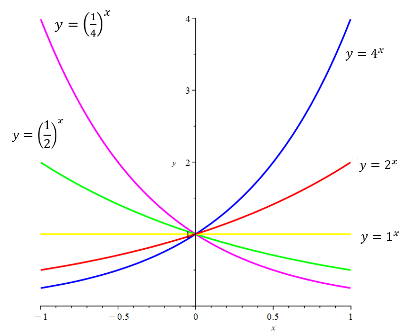
Both the red and blue curves above are examples of exponential growth because their base is greater than 1. The green and purple curves are examples of exponential decay because their base is between 0 and 1. The yellow curve is a special case, and we won’t consider this further, since it can be classified as a linear model.

The Natural Exponential

If you study calculus, you’ll find that the most convenient base for the exponential is Euler’s number, which is denoted by the letter $e$. This gives us the natural exponential function $y=e^x$.

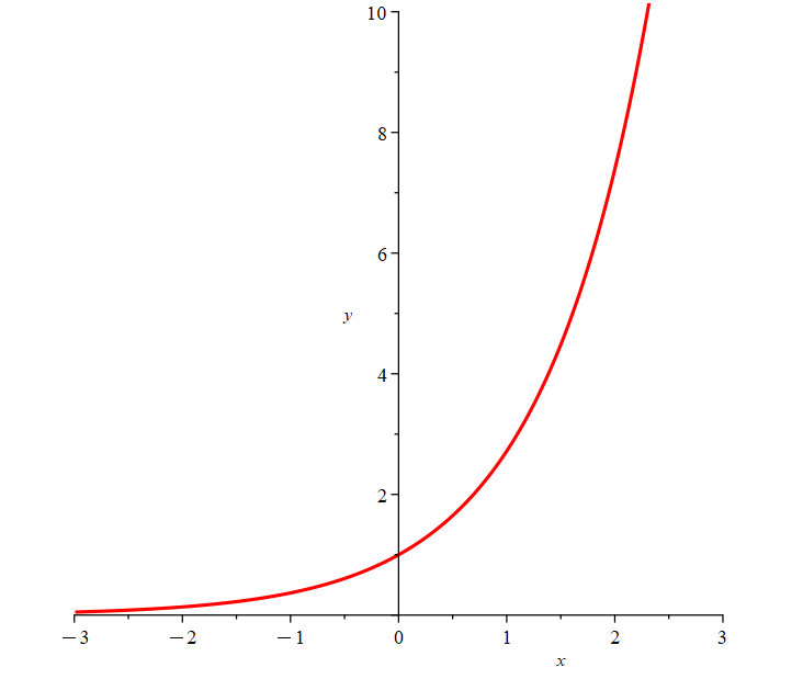
Euler’s number, $e$, is the number such that  $\underset{h\to 0}{lim}\frac{e^h-1}{h}=1$ 
                                                                         h → 0                                         
(ie., as $h$ gets smaller, the function $(e^h-1)/h$ approaches 1) and has a value such that $e=2.71828$.

Logarithmic Functions

The inverse of an exponential function is called a logarithmic function. Therefore, the inverse of $f(x)=a^x$ is the logarithmic function with base $a$, such that $y={\log }_{a}x⟺a^y=x$.

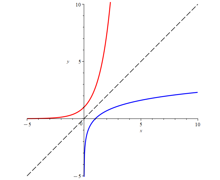
In the figure above, the red line represents an exponential function and the blue line represents its inverse, the logarithmic function. Since the exponential and logarithmic functions are inverse functions, cancellation laws apply to give:

${\log }_a{a}^x=x$ for all real numbers $x$

$a^{{\log }_{a}x}=x$ for all $x>0$

The Natural Logarithm

We already stated that e is the most convenient base to work with for exponential functions. The same is true when working with logarithmic functions. The logarithmic function with base e is called the natural logarithm and is denoted by the special notation:

${\log }_{e}x=\ln x$

Now, the same cancellation laws can apply for the natural logarithm, such that:

$\ln e^x=x$ for all real numbers $x$

$e^{\ln x}=x$ for all $x>0$

Finally, note that the logarithm and natural logarithm functions are related by the following change base formula:

${\log }_{a}x=\frac{\ln x}{\ln a}$, where $a\ne 1$